Gaussian Processes

A fundamental aim of the Physical Sciences is to be able to make useful predictions about the world around us. Predictions can be made by leveraging relationships between the different quantities that describe the state of a physical system which are often inferred empirically via observation of the system in different states. In the Earth Sciences, the physical systems we wish to model are often highly complex and, as such, require high-performance computer technology in order to solve numerical implementations of the physical relationships that we have derived.

Common research questions in Earth Sciences require not one but many predictions of different system states. In numerical modelling, such experiments are known as large ensembles and can be used in such applications as: assessing the uncertainty in a particular model prediction; understanding the importance of each of our inputs in determining our model output (known as sensitivity analysis); or finding the best fitting model to known data. Experiments like this can quickly become infeasible to perform using traditional computational methods when the required ensemble sizes are too large, but what if we could predict the outcome of a computer simulation without ever having to run it?

A Gaussian Process (GP) is a valuable machine learning tool that can be used to predict the relationship between data points, a problem known as regression, and make predictions in a fraction of the time taken to run most numerical models. GPs also provide key advantages over classical solutions to the problem of regression. Firstly, they don’t require prior assumptions to be made about the form of the relationship between input and output that classical fitting (such as linear, exponential or quadratic) fitting would do, as shown in Figure 1. Instead, GPs generate the most likely function from the infinite set of possible functions that fit both our data and our beliefs about the function’s characteristics. Secondly, a GP is able to provide an estimate of the uncertainty of the predictions it makes, with uncertainty typically being higher where we have fewer data points available.

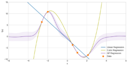
Figure 1: A comparison of fitted functions produced by two common types of regression, linear and cubic, alongside a GP regression when applied to sample data. We can see that, owing to our specified prior beliefs, the Gaussian process has not made rigid assumptions about the shape of our function and provides uncertainty in our data.

For numerical modelling in the Earth Sciences, GPs present a fantastic tool for overcoming the computational cost of running large ensemble experiments. In this instance, when the data points we provide are the inputs and outputs of a numerical model, we refer to this GP as an emulator. By training our GP on a small subset of model outputs from simulations that we have run, we can sample further outputs from our GP in place of running new models and be provided with both a best estimate and uncertainty in our emulated model prediction. We commonly choose to perform this training directly on diagnostics of interest derived from our model output, as illustrated in Figure 2.

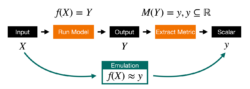
Figure 2: GPs are commonly applied to the challenge of model emulation. By training a GP emulator on a small subset of model outputs it is possible to predict diagnostics for new models which have not yet been computed.

GPs are a powerful, flexible, and robust machine learning technique applied widely for prediction via regression with uncertainty. Implemented in packages for many common programming languages, GPs are more accessible than ever for application to research within the Earth Sciences.

Using GPs to Emulate an Ice-Sheet Model

An example of GPs applied to numerical modelling can be found in a recent ice-sheet modelling paper titled: “Quantifying the Uncertainty in the Eurasian Ice-Sheet Geometry at the Penultimate Glacial Maximum (Marine Isotope Stage 6)”. In this work, aimed to better understand sea-level change during the Last Interglacial (LIG) - the last time in Earth’s history that the Greenland and Antarctic ice sheets were smaller than today – focussed on improved predictions of future ice sheet melt scenarios in a warming world. Sea-level records during the LIG are affected by the large Eurasian ice-sheet that existed prior to the Last Interglacial. Here we utilised GPs to emulate regional ice-sheet volumes in order to understand the uncertainty in our ice-sheet models, and thus the effect this uncertainty may have on piecing together LIG sea-level records. Figure 3 shows the resulting probability distribution of total Eurasian ice-sheet volume, after we used GPs to perform a technique known as history matching to narrow down our range of outputs by using known observations.

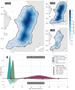
Figure 3. (a) Penultimate Glacial Maximum (PGM) Eurasian ice-sheet thickness ensemble member from the history matching ensemble with total ice-sheet volume closest to the probability distribution mean (48 m SLE). Smallest (b) and PGM largest (c) history matched ensemble members after history matching. (d) Probability density functions of unconstrained (bottom, lighter shade) and history matching constrained (top, darker shade) ice-sheet volumes for ensembles of the 20 ka GLAC-1D (blue) and 22 ka ICE-6G Last Glacial Maximum margins and the PGM (purple) compared against published ice-sheet dynamical simulations reconstructions from the corresponding time periods (Colleoni, 2009; Lambeck et al., 2006; de Boer et al., 2013; Peltier et al., 2015; Tarasov et al., 2012). Dashed grey line shows alternative probability density function when we constrain to simulations with ≤ 5 km maximum thickness.

You can read more about this work here:

Pollard, O.G., Barlow, N.L., Gregoire, L., Gomez, N., Cartelle, V., Ely, J.C. and Astfalck, L.C., 2023. Quantifying the Uncertainty in the Eurasian Ice-Sheet Geometry at the Penultimate Glacial Maximum (Marine Isotope Stage 6). The Cryosphere Discussions, pp.1-31. DOI: https://doi.org/10.5194/tc-2023-5.